Example

Below is an example showing how to use the the simulator class to simulate a realistic microlensing event at a randomly drawn sky position.

The first step is to extract the planned cadence given a single bandpass and RA/DEC in decimal degrees.

from rubin_lc_simulator import simulator

# Will simulate i-band data
band = 'i'

# Helper function to draw LSST sky positions (only those for which airmass < 1.4)
ra_dec = simulator.draw_random_coord()

# Initiate the class instance with the positions and bandpass
lsst_simulator = simulator.LSSTSimulator(ra=ra_dec[0], dec=ra_dec[1], band=band)

# Extract the spatial slicer the rubin_sim API uses to evaluate the sky on the spatial grid
dataSlice = lsst_simulator.LSST_metrics()

# Can now simulate the cadence
mjd = lsst_simulator.lsst_real_lc(dataSlice)

With the cadence saved, we can now simulate the lightcurve using any model that works with adaptive cadence. IMPORTANT: The mjd as output above may not be sorted, this is by design. When used to simulate your lightcurves you must ensure no sorting occurs, and that the magnitudes you simulate are according to this unsorted array!

For this example we will use the built-in lightcurves module which includes a function to simulate microlensing events (PSPL). This function returns the simulated magnitude as well as the event parameters, but note that the simulator only requires the magnitudes.

from rubin_lc_simulator import lightcurves

# Draw a random baseline using the built-in function, which draws randomly according to the saturation and 5sigma depth limits.
baseline = simulator.draw_random_baseline(band)

# Simulate the lightcurve
mag, u0, t0, tE, blend_ratio = lightcurves.microlensing(mjd, baseline)

With the cadence-dependent magnitudes simulated, we can now simulate the per-epoch errors and add noise to each point. This is done via the lsst_real_lc class method, which takes as input the extracted dataSlice as well as the simulated magnitudes from your model. This method will assign the mjd, mag, and magerr attributes. These will be sorted by timestamp. Important to remember that the input mag must not be sorted as it must correspond to the initially ouput mjd.

# The following class method will simulate the errors and assign the lightcurve attributes (mjd, mag, magerr)
lsst_simulator.lsst_real_lc(dataSlice, lc=mag)

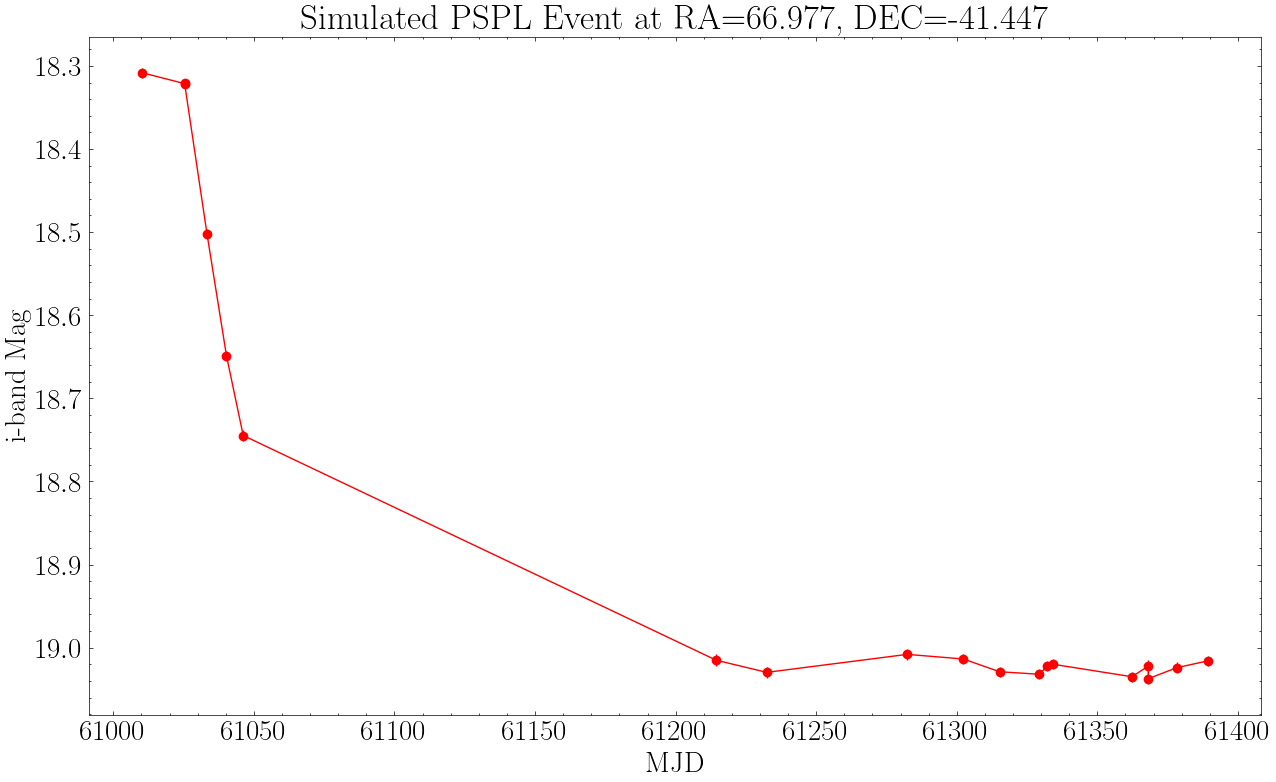
# Plot
import pylab as plt

plt.errorbar(lsst_simulator.mjd, lsst_simulator.mag, lsst_simulator.magerr, fmt='ro-')
plt.gca().invert_yaxis()
plt.title(f'Simulated PSPL Event at RA={ra_dec[0]:.3f}, DEC={ra_dec[1]:.3f}')
plt.xlabel('MJD'); plt.ylabel(f'{band}-band Mag')
plt.show()